Converse, as a multi-scale material modeling software, offers other useful tools besides the easy generation of anisotropic material cards. The material editor in Converse and S-Life Plastics, for example, allows the degree of anisotropy of a material or component to be assessed in a vivid way. Simple quasi-isotropic material cards can also be created and exported for initial estimative analyses. This allows comparative analyses without already having a fiber distribution. In the following, some basic terms in the context of anisotropy of injection molded short fiber reinforced plastics will be briefly explained first. Subsequently, it is described how the "Composite Calculator" and the "Polar Diagram", which is new from version 1.5 of the PART Software Package, can be used beneficially.
Material and component properties
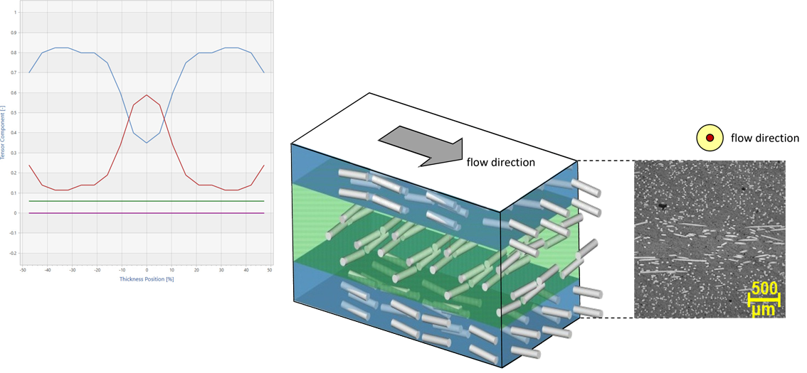
In the case of short-fiber-reinforced plastics, as with long-fiber-reinforced and continuous-fiber-reinforced materials, it is not really possible to speak of material properties. Rather, they are component properties, since the "material" is not created until the component is manufactured. A characteristic feature of fiber-reinforced materials is their layer structure. While this is intentionally designed into the component in the case of continuous fiber-reinforced materials, it is formed in the case of injection-molded short fiber-reinforced materials as a result of the flow processes during mold filling (Fig. 1). The mechanical properties of the "individual layers" superimposed over the component thickness then correspond to the material or component properties at this point. These are so-called homogenized properties, since no distinction is made between the individual components of the composite, i.e. fiber and matrix, and the layers.
Orientation tensor and fiber orientation
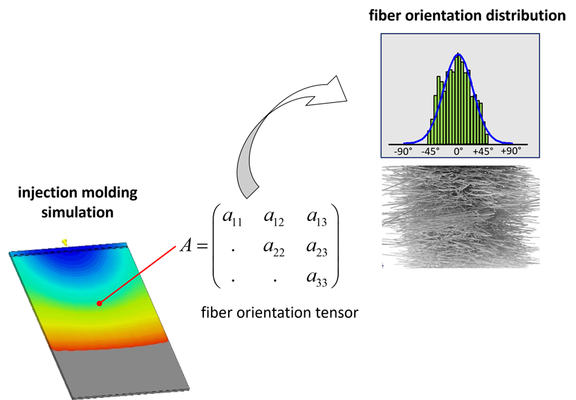
To determine such homogenized mechanical properties, knowledge of the local microstructure, i.e. in this case the fiber orientation, is required. This is then incorporated into the multiscale material model, which homogenizes the real heterogeneous material. Details will not be discussed here. The fiber orientation can be determined experimentally, e.g. by means of µCT measurements (Figure 2).
Of course, this already assumes the existence of a component. Therefore, the fiber orientation distribution is usually determined numerically by means of an injection molding simulation. However, the injection molding simulation provides the fiber orientation distribution only indirectly via the orientation tensor. The spatial distribution of the fibers must be reconstructed from the orientation tensor using suitable mathematical methods (Figure 2). One problem here is that the orientation tensor does not allow any statement about a unambiguous fiber orientation distribution, in the sense of an angular position of the individual fibers with respect to a reference coordinate system.
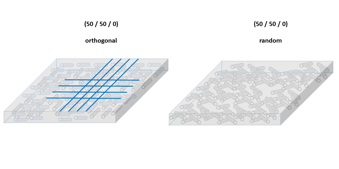
Figure 3, for example, shows two different fiber orientations, both of which can be described by the identical orientation tensor (a1|a2|a3 = 50|50|0). Mechanically, however, the two fiber orientations are different. For example, if we consider the direction-dependent stiffnesses, the orthogonally oriented fibers have identical properties only in the 0° and 90° directions, while the plate with the fibers randomly distributed in the plane has identical stiffnesses in each plane direction. The mathematical procedure used to calculate the orientation tensor back into a fiber orientation distribution should take this relationship into account. One assumption that can be usefully made here is that as few assumptions as possible are made in advance about the orientation of the fibers, while at the same time the resulting fiber orientation distribution is in agreement with the orientation tensor measured or obtained from the injection molding simulation. This corresponds to a so-called "maximum information entropy" state. In other words, this means that the simplest model out of a number of possible models has to be selected, which describes the given state without contradictions. In PART Engineering software, for this reason, the so-called "maximum entropy method" is used to reconstruct the fiber orientation distribution from the orientation tensor. The method usually provides very good correlations between calculated and measured fiber orientation distributions [1].
Composite Calculator: Helpful tool for plausibility checks and simple analyses
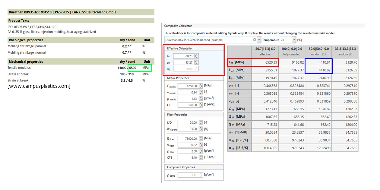
The basic relationships described above are reflected in the material editor of Converse and S-Life Plastics in the Composite Calculator. This tool, allows a quick analysis of the effect of different fiber orientation distributions on the anisotropic mechanical properties. Figure 4 shows a screenshot of the Composite Calculator.
The overview table shows the nine stiffness properties of the anisotropic material and the three coefficients of thermal expansion. These are calculated via the internal multiscale model for different values of the orientation tensor in each case. The values of the orientation tensor can be freely entered as eigenvalues or principal values (a1|a2|a3) on the left (Figure 4, red). Of special importance here is the so-called "effective orientation". This is the constant orientation averaged over the wall thickness of a specimen, for example, which leads to identical stiffnesses (tensile moduli) as the actual inhomogeneous distribution of the fiber orientation (Figure 1, left). One can adjust the effective orientation so that the value of E11 (tensile modulus in the principal orientation of the distribution) approximately corresponds to the tensile modulus parallel to the flow direction measured in tests or taken from a database (E11 = E0, Figure 4, red = green). Then this orientation found is a good estimate of the orientation state in the sample, without the need for CT measurement or injection molding simulation. Or the other way around, if the orientation tensor is known from a measurement or injection molding simulation, the anisotropic mechanical properties can be determined directly for this position in the component. Both procedures can be useful in a simple way in the context of plausibility checks.
Furthermore, the Composite Calculator shows the corresponding mechanical properties for certain distinguished orientation states in columns. This is the fully oriented state (100|0|0) as the extreme state when all fibers are aligned exactly in one direction, which in fact never occurs in injection-molded short-fiber-reinforced components. As well as the states of maximum random distribution in plane (50|50|0) and in space (33|33|33). The Random 3D state thus corresponds to a quasi-isotropy, with identical properties in all directions. However, since injection molded components tend to have a planar fiber orientation distribution due to the predominantly laminar flow of the plastic melt, Random 2D is more relevant.
It is known from practice that, with respect to a component's basic stiffness, the use of a tensile modulus measured in the direction of flow of the melt, e.g. from a database, provides component stiffnesses that are too high for a simplified isotropic FEM analysis. For this reason, an empirical reduction factor for the tensile modulus is often used in practice, with which the nominal tensile modulus from the data sheet is reduced to approx. 65-70 %. It has been shown that for typical technical components (glass fiber weight fraction 20-50 %, wall thicknesses 3-4 mm, mostly flexurally dominated load) the basic component stiffness can be reproduced well in many cases. However, this applies exclusively to the stiffness, not to the strength and to components that do not show a pronounced fiber orientation in the load direction.
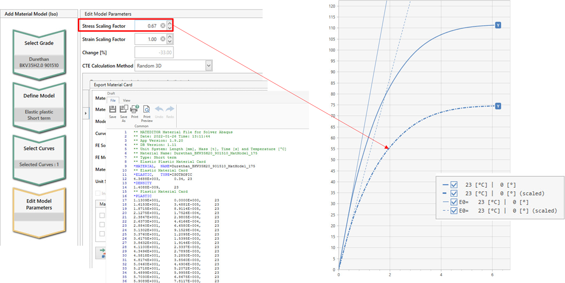
The stiffnesses determined in the Composite Calculator for the Random 2D state parallel and perpendicular to the principal fiber orientation (E11 and E22) can now be used to determine a material-specific value for such a reduction factor. Figure 4 (blue) shows, for example, a tensile modulus E11 = 4411 MPa for the random 2D state. A tensile modulus E0 = 6500 MPa is taken from a database (Figure 4, green). If both values are put in relation to each other, a factor of approx. 0.67 is obtained in the example here. This approach often yields values with a surprisingly good agreement with the empirical reduction factor already mentioned in practice.
This value can be used as a scaling factor to scale the entire stress-strain curve. This can also be done in the Material Editor using the Stress Scaling Factor when defining isotropic material cards (Figure 5). As already mentioned, this is only a rough estimate in terms of a basic component stiffness, a strength assessment based on such a scaled curve should not be conducted.
Finally, the material cards with the scaled curve can be exported directly in the respective solver syntax. For initial estimative analyses, this is an easy way to work with isotropic material models to perform comparative analyses without already having a fiber distribution.
Polar diagram: Fast evaluation of the influence of fiber and load direction
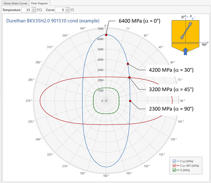
In the case of anisotropic materials or components, it is important to know how the fiber direction and the load direction are aligned to each other in order to evaluate the mechanical situation at a specific position in the component. As shown above, this determines stiffness and strength. As of version 1.5 of the PART Software Package, a polar diagram can be used to evaluate this influence in a simple way. Figure 6 shows an example of a polar diagram for a PA66+GF35.
The 0° direction here corresponds to the inflow direction of the test specimen or plate. The stiffnesses (tensile and shear moduli) of the composite material can be read off concentrically for different load or cutout positions. For example, at an angle of 0° the tensile modulus is approx. 6400 MPa, while at 90° the modulus is only approx. 2300 MPa.
It is interesting to look at an angle of 45°, where a tensile modulus of approx. 3200 MPa is obtained. When determining anisotropic material properties, an angle of 45° to the direction of flow is often used in order to have a further reference point for the material properties in addition to the extreme angular positions 0° and 90°. The polar diagram now shows very clearly that the tensile modulus to be expected at 45° does not lie midway between the extremal positions, but is closer to the 90° position at 3200 MPa. The central value of approx. 4350 MPa is better approximated by a cutout position of 30° (4200 MPa). This would therefore be more favorable in terms of calibration of an anisotropic material model. This result, determined here by Converse purely by calculation, has also been confirmed experimentally in tests on comparable materials.
[1] Breuer, K.; Stommel, M.; Korte, W.: Analysis and Evaluation of Fiber Orientation Reconstruction Methods. J. Compos. Sci.2019, 3(3), 67, https://doi.org/10.3390/jcs3030067
Author
Dr. Wolfgang Korte is Managing Director at PART Engineering GmbH, Bergisch Gladbach, Germany