What is Multiscale Modeling?
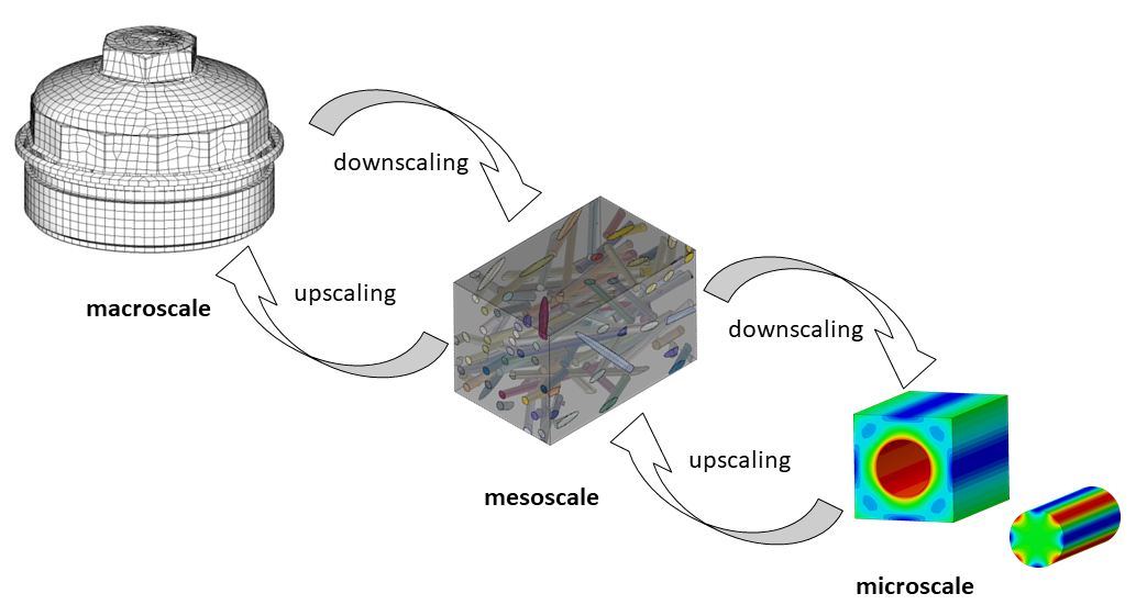
Multiscale modeling approaches are increasingly used in structural simulation. By means of such approaches, the material behavior of inhomogeneous materials can be described. In particular, such models are used for injection molded short fiber reinforced plastics. The idea here is to resolve the complex material structure in the component by changing the length scale range (localization or downscaling) to such an extent that the relationships in the higher-resolution length scale range (micro or meso level) are more accessible to a mathematical description (Figure 1).
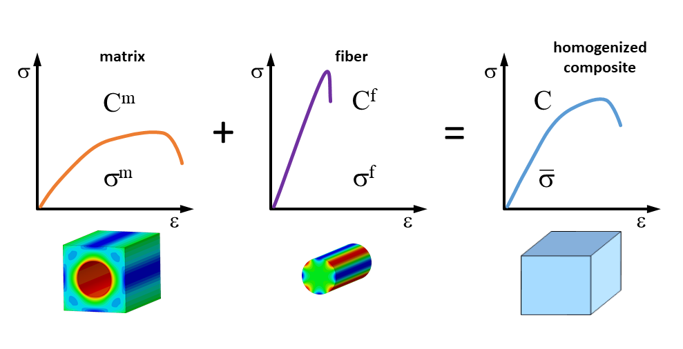
Thus, it is possible to calculate the behavior of a composite material only on the basis of the material properties of its constituents, i.e. matrix polymer and reinforcing fiber. The constituents with their specific properties and their spatial configuration then determine the material behavior of the composite also at the macroscopic component level (Figure 2).
For reasons of efficiency, it is now not appropriate to represent a complete component by completely modeling its microstructure. For this reason, a so-called homogenization (upscaling) is carried out. Starting from the properties of the inhomogeneous material at the micro or meso level, equivalent homogenized properties (e.g. stiffnesses) are determined. The material is then regarded as a homogeneous continuum. In the case of short fiber reinforcement, the homogenized material then exhibits analogous anisotropic behavior as the real inhomogeneous composite material. The homogenized material characteristics can then be used to perform numerically efficient FEM analyses of the component. The material modeling at the micro or meso level including the homogenization can be done in different ways. This is the main difference between the various multiscale modeling approaches. In the following, some of the frequently used approaches are presented.
Various Multiscale Approaches
The basis of the approaches is the definition of a so-called representative volume element (RVE). The RVE represents a cutout of the macroscopic component structure. On the one hand, the RVE must comprise the typical microstructure of the material to such an extent that, when the volume section is further enlarged, its external mechanical properties no longer change. It must be representative in a statistical sense, i.e. it must allow a reasonable averaging in the considered section. On the other hand, the RVE must be smaller than the characteristic dimensions of the component. As a rule, several RVEs must be defined for a component, since the local microstructure in the component also differs as a result of the fiber alignment. Basically, the multiscale modeling approaches can be divided into numerical and analytical procedures. Both approaches are presented in the following as examples.
Numerical Multiscale Approaches
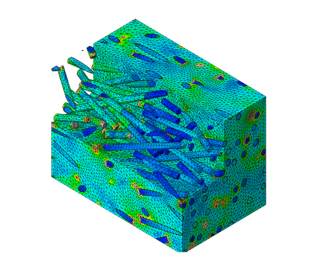
Numerical multiscale models represent the real microstructure on the meso level in a defined section of the component, the RVE (Figure 3). FE models are typically used for this purpose. The challenge here is to model the microstructure with sufficient accuracy while keeping the model size within acceptable limits. For the model to be representative of the component section under consideration, a sufficient number of fibers must be modeled, e.g. 100 fibers. These are then randomly distributed in the volume according to the assumed spatial fiber orientation distribution (angle classes). Periodic boundary conditions are imposed on the bounding surfaces of the RVE. The displacement boundary conditions of the respective opposing surfaces of the RVE are coupled. This satisfies the assumption that the cutouts of the microstructure line up in the component.
Macroscopic displacements can now be imposed on the RVE, which are obtained from the corresponding position in the component via an FE analysis. Again, by means of an FE analysis of the RVE, the strain and stress distribution in the RVE is determined. In a further step, homogenization is then performed via volume averaging of the strain and stress distribution in the RVE:
 (1)
(1)
with: ε strain tensor, σ stress tensor, V volume, ( ¯ ) volume averaged values
This then gives the averaged stiffness tensor:
 (2)
(2)
with: C volume averaged composite stiffness
This can then be transferred back to the FE simulation of the component to calculate the next load step.
Due to the nested FE analyses of component and RVE, the term FE2 is used for this procedure. This already indicates the high numerical effort. For this reason, different variants of the procedure were developed. In the case of linear-elastic material behavior, the stiffness tensor does not change over the load steps. In this case, it is possible to work with pre-analyzed RVEs whose stiffnesses are then stored in a database and assigned to the respective local microstructure in the component. Instead of an FEM analysis of the RVE, it is also possible to work with a voxel-like structured mesh that is calculated using a so-called FFT solver. This can significantly reduce the computation time for the RVE. There are also approaches that use numerical RVEs to train a neural network (AI). The neural network then provides an analytical model for the mechanical behavior of the RVE, which can be efficiently passed to the simulation of the component [1].
Numerical RVEs have basically no limitations in terms of material description. In addition to linear-elastic material behavior, plastic and viscoelastic behavior can also be described. Furthermore, a high resolution with regard to the cause and localization of damage can be achieved within the scope of failure evaluation. For example, it is possible to differentiate between fiber fracture, matrix fracture and fiber/matrix debonding. The price for this, however, is the high modeling effort and very long computing times, so that an analysis of complete components with this approach is not suitable for practice, at least at present.
Analytical Multiscale Approaches
Historically, the analytical multiscale approaches known today are based on micromechanical models that have been known for many decades. Here, too, all methods aim to homogenize a physically inhomogeneous material and to provide averaged mechanical properties that exhibit equivalent behavior as the inhomogeneous material. In connection with analytical multiscale approaches, this is also referred to as mean-field homogenization (MFH). This expresses the fact that mechanical field quantities such as strain and stress are averaged in the RVE to calculate the effective stiffness of the homogenized composite.
Mixing Rules
The simplest models are mixing rules that calculate the stiffness or compliance of the composite from the fiber volume fraction and the stiffnesses of fiber and matrix. The approaches of Voigt and Reuss are worth mentioning here:
![]() (3)
(3)
![]() (4)
(4)
with:
C stiffness tensor, ![]() compliance tensor, νf fiber volume fraction, νm = (1-νf) matrix volume fraction
compliance tensor, νf fiber volume fraction, νm = (1-νf) matrix volume fraction
Since the fiber weight fraction is usually better known, the fiber volume fraction can be calculated as follows:
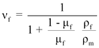 (5)
(5)
with: μ fiber weight fraction, ρ density
Voigt's approach assumes that fiber and matrix experience identical strain in the RVE, whereas Reuss assumes identical stress. Voigt therefore calculates the stiffness of the composite, while Reuss calculates the compliance. The Reuss approach is also known as the inverse mixing rule. Since no information about the fiber geometry is included in either model, they are only rough approximations for geometrically oriented (non-spherical) inclusions. The Voigt approach is an upper bound and the Reuss approach a lower bound for the composite stiffness.
Models Based on the Eshelby Theory
A number of more powerful models exist than the mixing rules described above, which can also take into account different fiber geometries and allow significantly better predictions of the composite properties even of anisotropic materials. Among the best-known models are those based on the work of Eshelby (1957). The starting point of Eshelby's theory is an RVE consisting of an ellipsoidal inclusion, in the case of short fiber reinforced plastics, a single fiber surrounded by an infinitely extended matrix.
A fundamental concept of the theory is the introduction of so-called strain and stress concentration tensors A and B. These are the ratios between the averaged strain (stress) in the fiber and the corresponding averaged values in the composite:
![]() (6)
(6)
![]() (7)
(7)
with: A strain concentration tensor, B stress concentration tensor
The concentration tensors A and B have the task of transforming the macroscopic external ![]() strains and stresses
strains and stresses ![]() at the boundary of the RVE to the local averaged strains
at the boundary of the RVE to the local averaged strains ![]() and stresses
and stresses ![]() in the fiber. The averaged composite stiffness can then be calculated using the following relationship:
in the fiber. The averaged composite stiffness can then be calculated using the following relationship:
![]() (8)
(8)
The volume-averaged stiffness C of the composite is calculated in this way from the known stiffnesses for fiber and matrix material Cfand Cm, the fiber volume fraction νf and the concentration tensor A. The only question that remains is how to determine the concentration tensor A. The literature provides various procedures for this.
Eshelby gives the strain concentration tensor A as follows.:
![]() (9)
(9)
with: I identity tensor, E Eshelby tensor
The Eshelby tensor E is calculated from the known values of the stiffness tensor of the matrix Cm and the length/diameter ratio of the fiber. Thus, all quantities for the calculation of the composite stiffness are known. However, the calculation of the composite stiffness by means of the strain concentration tensor AEshelby is only accurate up to fiber volume fractions of approx. 1 %. In this context, one therefore also speaks of the dilute Eshelby model. Consequently, this is not directly applicable to short-fiber-reinforced plastics of practical relevance.
For this reason, Mori and Tanaka proposed an alternative definition of the strain concentration tensor A for non-dilute materials, which is frequently used for modeling short-fiber-reinforced plastics. The basic idea of Mori and Tanaka is that a fiber around it sees only properties of the matrix and not those of the homogenized composite (see Eq. (6)):
![]() (10)
(10)
Thus, the fibers are so far apart that they have no interaction with each other. Using Eshelby's fundamental solution for the mechanical relations of a single fiber embedded in an (infinitely extended) matrix, the strain concentration tensor AMT of Mori and Tanaka can be calculated under this assumption to:
![]() (11)
(11)
Using the strain concentration tensor AMT and Eq. , the stiffness of the composite material finally follows. The equation initially applies to any material behavior in fiber and matrix, since no restrictions have been made so far for the stiffness tensors Cf and Cm. Under the limiting assumption of linear-elastic material behavior, Tandon and Weng give an analytical solution with which the composite stiffness can be calculated directly in terms of the engineering constants. However, if, for example, the matrix is described elasto-plastically, an anisotropic stiffness tensor always follows in general. In this case, no analytical solution can be given, and the composite stiffness must be determined iteratively numerically.
A restriction of the Mori-Tanaka theory, and all relations based on it, which is significant for practical applications, is based on the assumption that a fiber is not coupled with a neighboring fiber. Thus, strictly speaking, the Mori-Tanaka approach applies only to low fiber volume contents. However, practice shows that the Mori-Tanaka approach can also be successfully applied for fiber volume contents of 30% and more.
Orientation Averaging
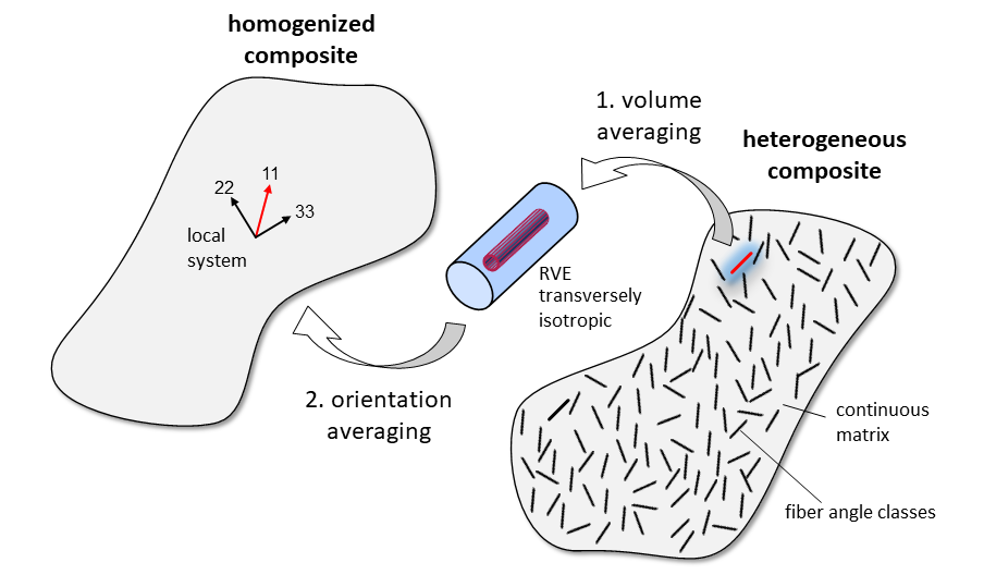
Since the Mori-Tanaka approach is based on the Eshelby solution, the relationship initially applies only to microstructures in which the fibers in the representative volume under consideration are all oriented in the same direction, i.e. unidirectionally (transversely isotropic). This is not the case for real microstructures in injection molded parts. Rather, there is a spatial fiber orientation distribution. In addition to the volume averaging of the composite stiffness shown above by means of the various methods, an averaging of the composite stiffnesses over the various fiber orientation angle classes must also be carried out in a second step. This is referred to as a 2-step homogenization. The result of both steps is the homogenized effective total stiffness of the composite for the given fiber orientation distribution (Figure 4).
The total stiffness of the composite is then calculated to:
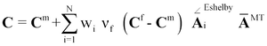 (12)
(12)
with: wi weight per angle class, ![]() strain concentration tensor transformed into local element coordinate system,
strain concentration tensor transformed into local element coordinate system, ![]() averaged strain concentration tensor
averaged strain concentration tensor
The weighting factors wi are obtained from the reconstruction of the orientation distribution function, which is further described below. The type of homogenization given in Eq. is called full-Mori-Tanaka homogenization in contrast to the so-called pseudo-grain homogenization. In pseudo-grain homogenization, not only the fibers are divided into different fiber angle classes, but also the surrounding matrix (grains). The strain concentration tensor is calculated independently of all other fibers. That is, coupling of the strain concentration tensor for each individual fiber to the situation in the surrounding composite is not considered. As a result, the interaction between fibers of different orientations is lost. In the full Mori-Tanaka formulation, on the other hand, the matrix is treated as a continuous phase. This seems to be closer to the real situation in the composite in terms of common sense.
Reconstruction of the Orientation Distribution Function
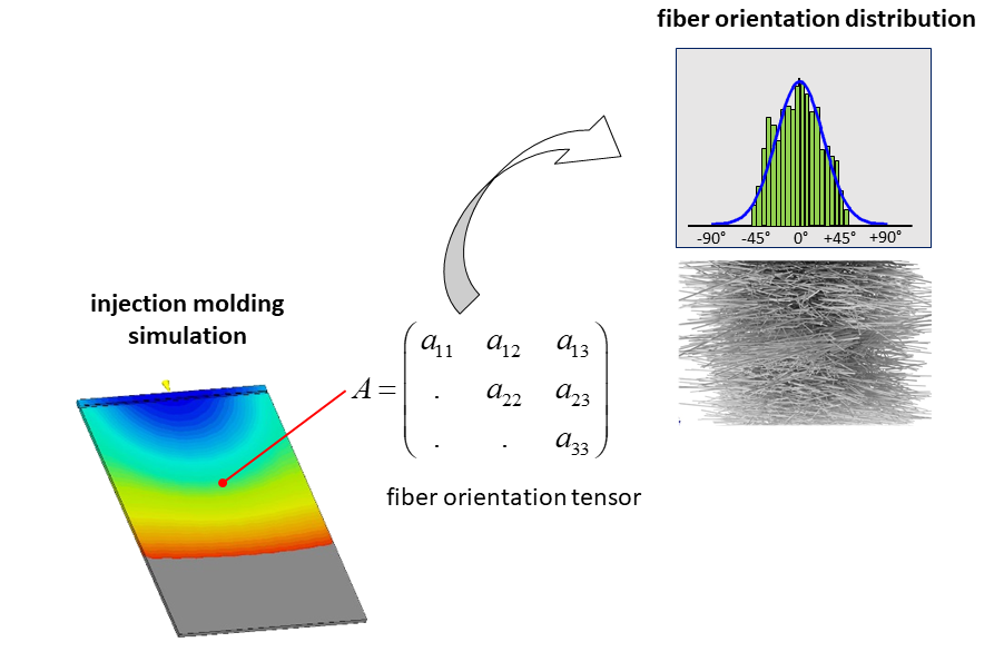
Both numerical and analytical multiscale models always require knowledge of the local microstructure in the component. This can be determined experimentally, e.g. by means of µCT measurements (Figure 5). Of course, this already assumes the existence of a component. Therefore, the fiber orientation distribution is usually determined numerically by means of an injection molding simulation. However, the injection molding simulation provides the fiber orientation distribution only indirectly via the orientation tensor. The spatial distribution of the fibers must be reconstructed from the orientation tensor using suitable mathematical methods [2] (Figure 5).
Conclusion
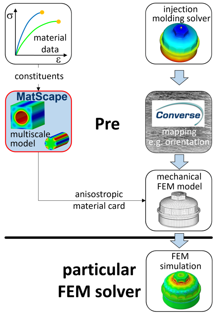
The 2-step homogenization based on the full Mori-Tanaka approach is implemented in PART Engineering's multiscale software Converse respectively the material modeling module MatScape for the determination of the linear elastic behavior of the composite. For the linear elastic case, such an approach is computationally very effective and provides the elastic properties in good agreement with experiments. However, for the plastic part of the material behavior, it is known that the predictive ability of analytical micromechanical models is generally poor. Moreover, accounting for plastic effects at the microscale implies an incremental numerical solution approach to the entire set of micromechanical equations, which is numerically very expensive. Therefore, plastic effects are accounted for in Converse by introducing an orientation-dependent yield criterion already defined for the homogenized composite, which is computationally very effective and easy to handle with respect to the calibration of the model. Thus, with the help of the analytical modeling approaches presented in this paper, so-called pre-homogenized material cards are computed which are then transferred to the respective FE solver (Figure 6).
Due to the performance of the hybrid approach implemented in Converse, the approach has already been implemented in a similar way by other authors [3]. This underlines the practical suitability of the PART software solutions.
[1] K. Breuer und M. Stommel, „Prediction of Short Fiber Composite Properties by an Artificial Neural Network Trained on an RVE Database“, Fibers, Bd. 9, Nr. 8, S. 14, 2021, doi: doi.org/10.3390/fib9020008.
[2] K. Breuer, M. Stommel, und W. Korte, „Analysis and Evaluation of Fiber Orientation Reconstruction Methods“, Journal of Composites Science, Bd. 367, Nr. 3, S. 22, 2019, doi: doi:10.3390/jcs3030067.
[3] H. Xu, M. Kuczynska, N. Schafet, F. Welschinger, und J. Hohe, „FE-based damage modeling approach for short fiber reinforced thermoplastics under quasi-static load coupling anisotropic viscoplasticity and matrix degradation“, Journal of COMPOSITE MATERIALS, Bd. 56, Nr. 20, S. 3113–3125, 2022, doi: DOI: 10.1177/00219983221109327.
Author
Dr. Wolfgang Korte is Managing Director at PART Engineering GmbH, Bergisch Gladbach, Germany