The simulation of long-term component behavior is often a challenge. On the one hand, this is due to the lack of material data and, on the other hand, to the lack of a suitable approach. This article shows how a meaningful simulation can nevertheless be carried out using simple methods and comparatively few material data.
Limited availability of material data
A qualified assessment of the behavior of the component under long-term loading is not possible without material data on the long-term deformation and possibly also failure behavior of the material. However, the availability of these input data is generally very limited. The reason for this is the huge effort required for their experimental determination. This is done by means of time-consuming and cost-intensive long-term creep tests. For the deformation behavior, several tests with a duration of 1,000 to 10,000 hours each (i.e. 1.5 months to slightly more than a year) are usually necessary. If necessary, the tests must be carried out at different temperatures. As a result, data on long-term behavior are only available for a few widely used standard commercial plastic grades.
Complex modeling of time-dependent material behavior
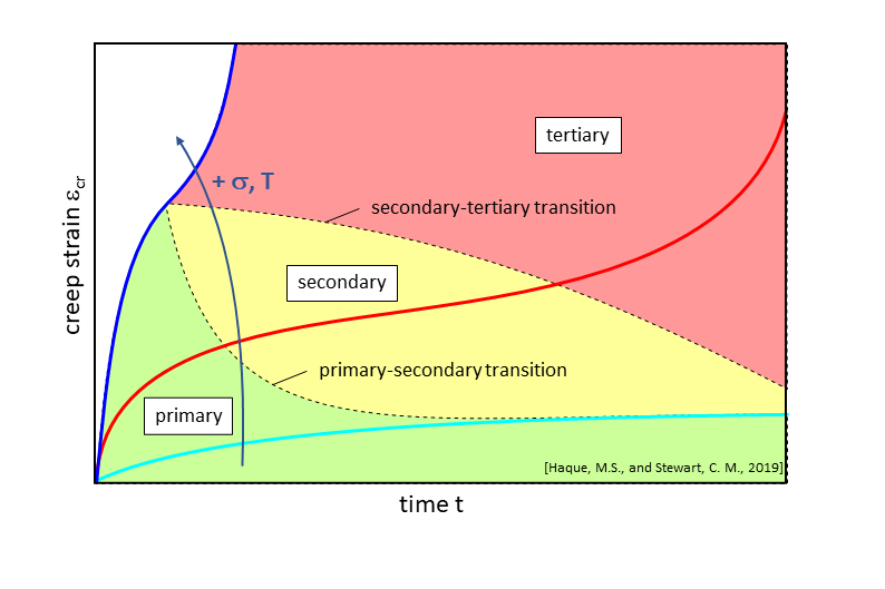
Plastics exhibit pronounced viscoelastic behavior, i.e. the response to a mechanical load depends not only on temperature but also on time. The time-delayed deformation due to a constant external load is referred to as creep. In particular, the time history of the strain is referred to as creep curve. A schematic creep curve up to failure is shown in Fig. 1.
The creep behavior can be divided into three phases:
- primary creep, degressive behavior, the creep rate decreases,
- secondary creep, the creep rate is almost constant and
- tertiary creep, progressive behavior, creep rate increases again until final failure (fracture or yielding).
With increasing temperature and creep stress, creep strain increases and duration to failure decreases.
The description of the creep behavior can be carried out with different mathematical models, often creep models are used. These assume that the creep strain εcr is made up of viscoplastic εv and plastic εpl strain components:
εcr = εvis + εpl
In addition, the short-time elastic behavior of the material εel can be defined by specifying a tensile modulus E. The creep strain is irreversible, after unloading only the elastic part of the strain resets, insofar as it has been defined. For this reason, the use of a creep model always has the limitation that only monotonically increasing load curves, i.e. no unloadings, can be described. A representation of the tertiary region of the creep curve (Fig. 1), i.e. the onset of failure, is also not possible with these models. The best-known creep models are the approaches according to Bailey-Norton and Findley [1], which are implemented in many FEM programs. The use of these models requires considerable expertise for the adjustment of the material model parameters.
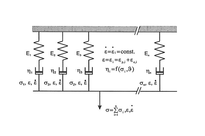
Furthermore, approaches exist to describe the long-term material behavior on the basis of rheological models. The long-term material behavior can thus be represented phenomenologically by means of corresponding parallel and series circuits of the basic rheological bodies spring, dashpot and friction element. These models exist in a wide variety of configurations. A well-known model for plastics is the generalized Maxwell model (Fig. 2).
The material behavior is represented by a parallel circuit of N spring-dashpot elements. In contrast to the creep models, unloading processes can also be represented in this way. Accordingly, they can be used for any long-term load characteristics, because the path dependence of the deformation behavior ("material memory") is captured. However, even such a model is only approximately suitable for comparatively low stresses, since linear material behavior (linear viscoelasticity) is assumed. In this respect, even this model cannot represent the complete creep behavior up to failure (Fig. 1).
A large number of extensions to this model exist, which are intended to take into account a wide variety of effects (nonlinearity, viscoelasticity, failure). However, the determination of the required model parameters is very complex. For example, if one assumes N=10 spring-dashpot elements, which is quite realistic, then it is already a matter of 20 model parameters that are required by fitting the model parameters to corresponding measurement data. If model extensions are added, there are even more. Even assuming that appropriate material data are available, such approaches are not practical in their present form. In addition, the question must be asked as to the benefit/effort ratio, since even with complex models not all effects are covered.
For this reason, alternative simple approaches are presented below which at least allow an estimate of the time-dependent material behavior and can be used in day-to-day business.
Practical approaches for the description of time-dependent material behavior
The approaches presented below are based on a creep modulus curve or an isochronous stress-strain diagram. For common plastic trade grades, there is a real chance that appropriate data are available from freely available sources, e.g. Campus [2].
Use of a creep modulus
The simplest material model thinkable is the Hooke model for describing linear-elastic behavior under short-term loading. Here, only a tensile modulus and the Poisson coefficient are required. The question arises as to whether such a simple model cannot also be used for long-term loading, if it is not the entire time history of the loading that is of interest, but only a specific point in time in the loading history.
In fact, the creep modulus Ecr can be used for this purpose. The creep modulus is the (fictitious) stiffness of a material assumed to be linear-elastic, which for the given creep stress leads spontaneously, i.e. without any time delay, to the same strain as the real viscoelastic plastic under the same constant creep stress after the loading time t. The creep modulus Ecr is the stiffness of a fictitious material assumed to be linear-elastic. However, to emphasize it again: Only the strain at the time considered is calculated. Loading and unloading processes cannot be described. A linear-elastic material model is thus misused, because for this particular boundary condition at a given time it provides the result we are looking for. However, the creep modulus as such is not present at any point of the component at any time. Neither is the real material behavior linear-elastic.
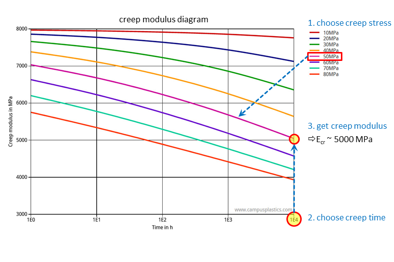
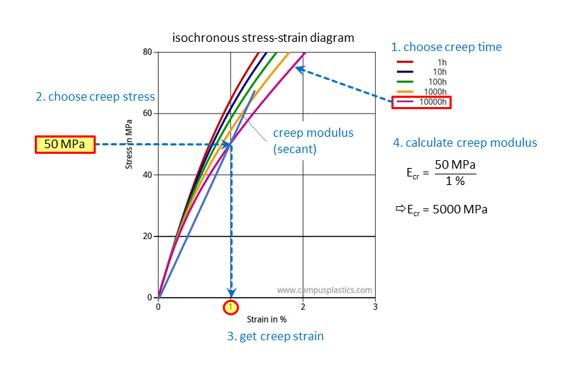
For this approach, the stresses prevailing in the component and the loading time must be known. The creep modulus can thus be read from the creep modulus diagram (Fig. 3). Here, the curve corresponding to the applied time-constant stress in the component must be chosen. Equivalently, the creep modulus can also be determined as the secant modulus of the isochronous stress-strain curve for the loading time and for the applied stress (Fig. 4).
In practice, the problem regularly arises here that there is not a homogeneous stress in the component, but an inhomogeneous stress distribution. This is not a problem if the maximum stress in the component is still approximately in the linear range of the isochronous stress-strain curve, or if the creep modulus curves for different stress values do not yet differ considerably. The creep modulus here is time-dependent but not load-dependent. The stress is in the linear viscoelastic range, so that a creep modulus accurately describes the strain distribution in the entire component. However, if the maximum stresses are above the linear range, then a creep modulus no longer accurately represents the strain in these areas. The following section explains a simple method for solving this problem.
Use of an isochronous stress-strain curve
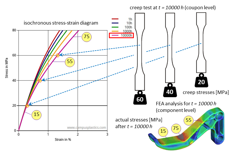
Analogous to the fictitious linear-elastic creep modulus, an elastic-plastic material model can also be used for estimating the long-term behavior. Let us look for the strain response to an arbitrary but temporally constant stress or the stress response to a temporally constant strain after a time t. If, as in the vast majority of cases, the stress in the component is not homogeneous and beyond the linear range, one approach could be to determine a separate effective creep modulus for each finite element. However, since the local stress is not known initially, the determination of the local creep moduli would have to be done iteratively. This approach is not practical.
However, from an isochronous stress-strain curve for a given time t, the strain response of the material can be read for any constant stress in time (Fig. 5). If such an isochronous stress-strain curve (for time t) is used as the basis for calibrating an elastic-plastic material model, this material model will provide the correct total strain for any stress at time t. This means, however, that the strain response of the material can also be read for the different stresses in time t. This means, however, that this approach also provides the correct strain responses at time t for the different stress levels present in a component that are no longer in the linear range. As with the creep modulus, a fictitious material behavior is assumed, in this case elastic-plastic.
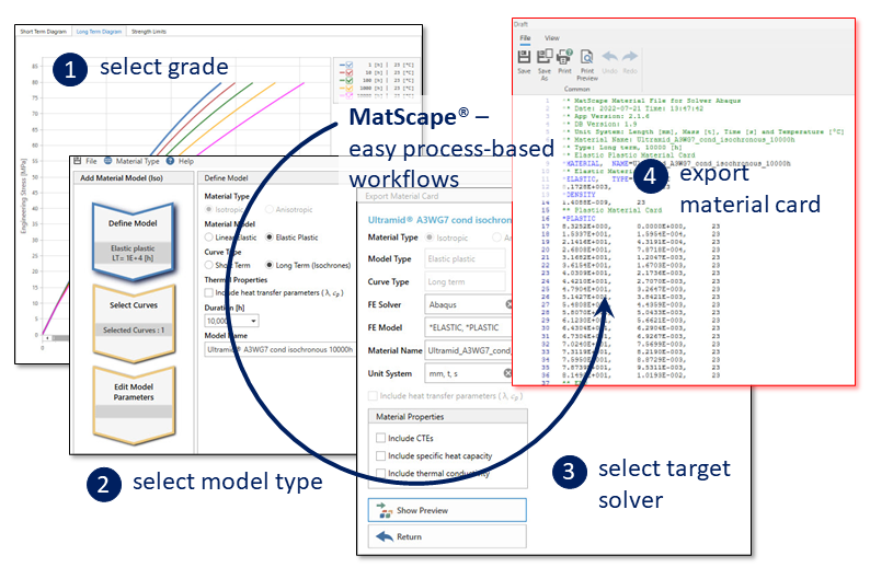
Using the MatScape material modeling module integrated in Converse and S-Life Plastics, the required elastic-plastic material cards can be easily exported directly from an isochronous stress-strain curve for various solvers (Fig. 6).
Thus, long-term behavior can be estimated after a time that corresponds to the curve being used. It is important to verify that the local stresses are constant over time at each point of the component during this time period, as these were the boundary conditions when the creep tests underlying the isochronous stress-strain curve were conducted (Fig. 5). A typical example where this is usually the case are components subjected to internal pressure.
Service life under long-term loading
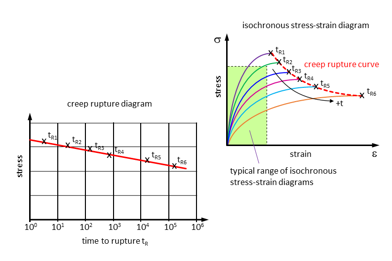
The higher the mechanical load or the resulting mechanical stress, the faster failure occurs. The plot of creep stress versus time up to failure is called the creep rupture curve (Fig. 7, left). However, isochronous stress-strain curves of the plastic trade grade, if available, are never shown up to failure, but only depict a limited subcritical strain range (Fig. 7, right). This regularly confronts the simulation engineer with the problem of assessing the determined stresses in terms of service life, even if they have been correctly determined using one of the methods described above.
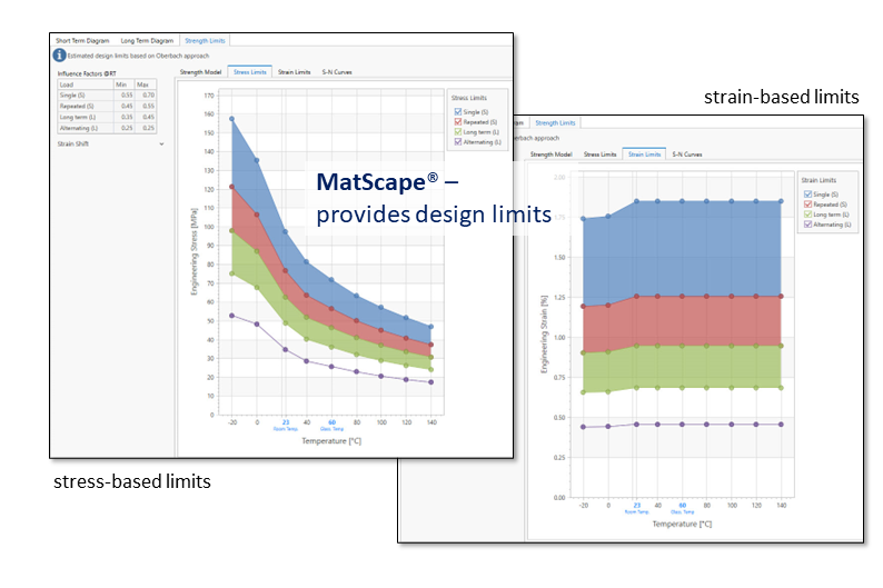
The MatScape material modeling module in Converse and S-Life Plastics solves this problem by allowing stress- or strain-based design limits for long-term stresses to be estimated at the push of a button for all plastic trade grades for which isochronous stress-strain curves are available (Fig. 8).
Conclusion
The effort required to experimentally determine creep curves and to calibrate sophisticated material models for long-term loading is considerable. In addition to time and money, the required expertise is often lacking. The simple approaches presented here are viable alternatives for estimating the long-term deformation behavior of plastic components.
For example, initial assessments can be made in the context of optimization or concept studies based on simple FEM analyses with linear-elastic or elastic-plastic isotropic material models.
Using the MatScape material modeling module integrated in Converse and S-Life Plastics, elastic-plastic stress-strain curves can be easily generated based on isochronous data. Long-term design limits can also be determined. In an ongoing publicly funded development project "Long-term material models for simulation", the models will be refined and implemented in MatScape in due course.
Thus, the software offers an easy-to-use approach to simulating plastic components subjected to long-term loading. Converse and S-Life Plastics can be purchased either directly through PART Engineering or can also accessed through the Altair Partner Alliance.
[1] M. Stommel, M. Stojek, und W. Korte, FEM zur Berechnung von Kunststoff- und Elastomerbauteilen, 2. Aufl. München: Carl Hanser Verlag, 2018. Available only in German language.
[2] N.N., CAMPUS - A material information system for the plastics industry.
Dr. Wolfgang Korte is Managing Director at PART Engineering GmbH, Bergisch Gladbach, Germany.