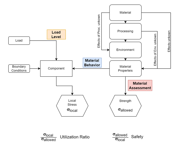
Figure 1 shows schematically the sequence of a typical strength assessment of a component. Geometry, boundary conditions and material behavior result in a stress distribution (stress or strain) in the component as well as its deformation. The evaluation is usually always carried out locally, which means that each point of the component is considered separately. The local stress must be set in relation to the strength of the material used. The strength has to be determined from the available material dates and, if necessary, corrected against the raw data as a result of different influences (e.g. processing influences, post-processing, aging, media influences, etc.). At the same time, the material model for the simulation must also be derived from the material data in order to calculate the stresses resulting from the load.
The quotient of calculated stress and the determined strength provides the degree of utilization, the reciprocal value can be interpreted as a safetyparameter. (By failure is meant here the local exceeding of the strength limit. This usually has nothing to do with the final component failure, especially for ductile materials.)
Figure 1 shows the three basic possibilities for targeted influence on the assessment result.
Known external influences that have not been considered in the material data have to be taken into account
Change of material behavior in the simulation model (material model)
Often there are no stress-equivalent tests of the material used. That are tensile tests carried out at the same temperature, strain speed/time, humidity (PA), media, etc. Such influences change the mechanical behavior of the material compared to the nominal from the data sheet of the raw material supplier. The best example is the local fiber orientations in GF-reinforced grades, which also influence the material behavior differently at each position of the component. In order for this changed behavior to be taken into account in the assessment, it must be included in the simulation of the component behavior. The material model used must therefore be adapted. This usually happens by converting (decreasing), capping or extending the stress/strain curve of the material via factors. Depending on the type of load case, this also results in different stress results, which can then be compared with corresponding strengths.
A risk assessment has to be carried out or uncertainties in the modelling have to be compensated
Reduction of strengths or increase of assumed loads
Safety factors are used as part of a risk assessment. This is where the probability of the occurrence of overload situations and possible damage consequences (system relevance, danger to life, etc.) are taken into account. Often, an increased load by an application-specific factor is assumed. With this load, higher degrees of utilization are determined and the component must be designed more conservative in order to pass the assessment.
As long as the material behavior up to failure can be assumed to be largely linear, this procedure is equivalent to a reduction in the assumed material strength. In the case of nonlinear material behavior, however, the two approaches can lead to completely different results. Here, an increase in the load due to the plastification of load-bearing cross-section of the component can lead to a complete failure (in the case of load-bearing capacity verification, this effect is just wanted), whereas a reduction in the assumed component strength does not show this effect.
The two approaches will be discussed using two exemplary load cases. This comparison should not be about distinguishing between right and wrong. Depending on the input data, question and experience with the specific component, each procedure can have its justification. Rather, it is about showing that there are always several ways to use reduction factors and that one must consciously distinguish whether a reduction affects the material behavior or the material evaluation and whether a reduction has local or global effects.
The first example is the frequently used snap hook, which is to be evaluated with regard to the assembly process. Questions are:
- Strength for one-time assembly
- Assembly force
The second load case is considered to be a container under internal pressure. This is about the assessment of strength of a burst pressure test (for a short time) at a given internal pressure. The assessments should be carried out on a stress-based basis.
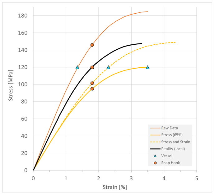
Figure 2 shows the different stress/strain curves used in this example.
From the database for the material used P(..) -GF30 read the orange curve marked with raw data.
The black curve represents the real local material behavior at the detection point, which unfortunately is unknown to all participants.
Both the raw data and the tests refer to short-term loads at room temperature. In this respect, therefore, no reduction is required. However, the load cases are simulated using an isotropic material model. According to experience, the stiffness should be reduced to 65% of the nominal value.
Two different curves are drawn in the diagram, because a reduction in stiffness can be achieved in several different ways. Here, on the one hand, all stress values were multiplied by the factor 0.65, alternatively the stresses were multiplied by the root of 0.65 and the strain was divided by the same value. The effect on the initial slope is the same, the yield curve is different.
As an alternative to adapting the material model, the load cases are calculated with the nominal stress/strain data (raw data) and the assumed strength is reduced afterwards for the assessment.
The different simulation results resulting from the use of the respective curves are marked by circles and triangles. As a displacement-controlled load case, the local strains for the snap hook are independent of the material model and thus also of a reduction in material behavior, but the assembly force changes. For the force-controlled internal pressure load case, on the other hand, the same stress values are calculated, regardless of the material, but the deformation of the container changes.
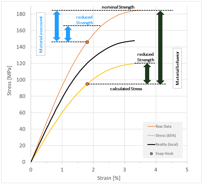
Load case snap hook
In the simplest case, the raw data is used directly for the calculation. The behavior of the material is not changed, instead the reduction takes place only during the assessment. A strength specific reduction factor can be used to reduce nominal strength. In Figure 3, this is indicated by the blue arrows. For the stress hot spot in the snap hook, it can be assumed here that the local fiber orientations are relatively similar to those in a tensile specimen (used for measuring the raw data) and the fibers are essentially aligned in the load direction. The use of the raw data to assess local strength is therefore quite appropriate. The locally calculated stresses are also valid, because the strain at the assessment point is independent of the material model. The amount of the reduction factor for the strength is not to be discussed here. However, it is important that this factor has nothing to do with the purely phenomenological 65% reduction in stiffness but should be specific for the evaluation of strength. For example, as a lower limit, the strength transverse to the fiber direction could be evaluated from corresponding tests. However, the use of the raw data in the material model also means that the calculated assembly forces are probably significantly too high.
The black arrows on the right side illustrate the procedure for reducing the material stiffness, i.e. the material behavior. The global reduction in stiffness also leads to a reduction in strength. At the same time, of course, the stresses calculated at the detection position are also reduced. Since all stress values of the curve were multiplied by the same factor, the degree of utilization does not differ from the blue procedure. The use of an additional, strength specific reduction factor is also possible.
The right black arrow relates the stress calculated with changed material behavior to the nominal strength. The reason here could be the same as above, namely that the material properties at the hot spot are similar to those in the tensile bar. This is not allowed here. The material can thus be significantly overestimated, as the calculated stresses are too low due to the reduction.
With the change in material behavior, however, the actual purpose of reducing stiffness was achieved here. The global component stiffness is better estimated with the reduced material model than would have been the case with the raw data. The assembly force is well predicted. (Not recognizable in the diagram ;-))
A sensible solution could be to first carry out the simulation with reduced stiffness in order to determine the assembly forces. Likewise, this simulation shows at least the location of the most stressed point on the component. If one can make an assessment of the local properties at this point, one should run a second simulation with a corresponding material model to evaluate the strength there.
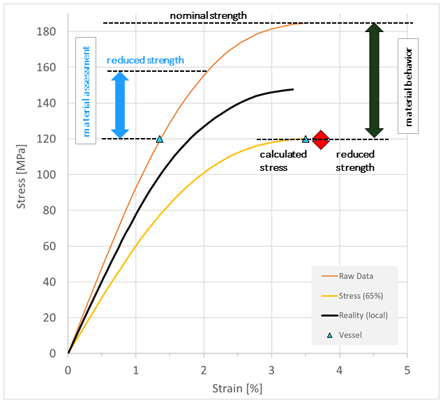
Load case pressure vessel
For the internal pressure loaded vessel, the calculated stresses are independent of the material model. On the stress side, therefore, in principle both the nominal and a reduced material model can be used. A special effect in this example is that the stress reaches the yield strength of the reduced material curve (see Figure 4). Should this state be reached for an entire component cross-section, a simulation would break off here. Even at lower stresses, the diagram shows the significantly higher plastic strain percentage in the reduced curve compared to the nominal one. The reduction, which should actually only concern stiffness, thus leads at the same time to an overestimation of the plastic strains. If the Pressure vessel would have to be designed for cyclic load this certainly would be an undesirable effect.
For both curves, a reduction only affects the strength side (see Figure 4). The factor of 0.65, which is actually related to component stiffness, also leads to a strength reduced by the same factor. Accordingly, the degree of utilization increases here by 1/0.65. In the example, this leads to a failure of the material at the detection point. Whether this reduction in strength compared to the data sheet is justified, the user can decide, but he should be clear about the effects of his approach.
With the given question about the strength of the container, nothing is gained by using a reduced material model. The calculated stresses do not change, the plastic strains are overestimated and convergence problems threaten. In addition, the stiffness-related reduction factor of 0.65 does not necessarily apply to the same amount for a reduction in stiffness.
Here, a sensible solution seems to lie more in the use of the raw data and the determination of a specific reduction factor with regard to strength.
It becomes clear in both examples that the use of reduction factors can lead to an overestimation of the component strength as well as to an underestimation or has no influence at all on the verification result. How a reduction is to be made in the context of the computational evaluation is not only a material-dependent question, but also always depends on the load situation and the question that is to be answered by a simulation.
Author
Dr. Marcus Stojek is Managing Director at PART Engineering GmbH, Bergisch Gladbach, Germany