Plastic components are often subjected to long-term loads. For the simulation of the behavior of such components, the correct application of suitable material models is fundamental. In practice, two problems frequently arise here: First, the procedure for determining the material model parameters is unclear. Second, long-term experimental material data are often not available in a suitable form, which is, however, a prerequisite for determining the model parameters.
In this article, the application of the Bailey-Norton material model is explained. The Bailey-Norton model is not the simplest possible model for long-term loading. In our blog article "Simulation of Long-Term Behavior of Plastic Components", more simple estimating methods are presented. However, sometimes it is essential that not only a deformation state at a certain point in time is sought, but the complete time-dependent deformation history. In these cases, the Bailey-Norton can be used under certain assumptions.
Understanding the Bailey-Norton Model
The Bailey-Norton model is commonly used for FEM simulation of the behavior of materials under long-term static loads. The advantage of the model is that it is usually standard in commercial FEM programs. The model is usually described mathematically in terms of the creep rate:
![]() (1)
(1)
Equation (1) represents the Bailey-Norton model in the so-called time hardening form. Alternatively, there is a strain hardening form equivalent in result, which will not be discussed further here. The model relates the applied stress to the strain accumulation over time. To determine the creep strain, the FEM program that is used integrates Eq. (1) over time:
![]() (2)
(2)
The model assumes that strain accumulation occurs as a power law of time with the exponent s. Furthermore, a dependence of strain accumulation on stress is given via the parameter n. The parameter A is a scaling parameter that shifts the strain on the y-axis. The model describes a nonlinear relationship between strain, stress and time. The terminology time hardening is derived from the fact that the strain shows a degressive course with increasing time (0 < s ≤ 1), i.e. the material deforms under-proportionally over time. In the case where s takes the value 1, a linear dependence of the strain on time is obtained. The creep rate is then constant per stress and the Bailey-Norton model turns into the Norton model, which is often used to describe creep processes in metallic materials. Due to its mathematical form, the Bailey-Norton model is suitable to represent the first and second creep phases (Figure 1). The model cannot describe the increase of the creep rate in the third creep phase until the onset of failure. This limitation of the range of validity has consequences for the determination of the model parameters and the interpretation of the simulation results, as will be shown below.
A step-by-step procedure for determining the model parameters and applying the model is presented below.
Step 1: Generation of the data basis
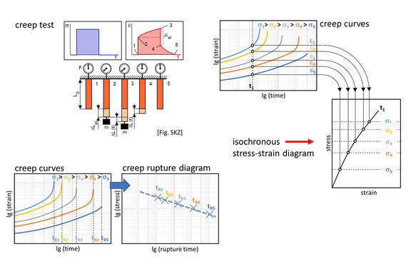
Ideally, from a creep test (Figure 2, top left), creep curves are available at at least two, ideally three, creep stresses (Figure 2, bottom left). In practice, however, this is often not the case for a given plastic grade. What does exist for some commercial grades [1], however, are the so-called isochronous stress-strain curves (Figure 3). These curves cannot be measured directly experimentally. Rather, they are obtained from creep curves by interchanging axis and curve parameters (Figure 2, right) [2]. In this respect, creep curves can again be obtained from an isochronous stress-strain diagram via the inverse procedure. Since the isochronous stress-strain curves are available for only a few discrete times (Figure 3), it is necessary to interpolate additional times in order to obtain a smooth curve of strain versus time. Such an interpolation usually has to be performed nonlinearly. Furthermore, in practical implementation it is advisable to describe the isochronous stress-strain curves first with a suitable analytical model in order to make interpolation and recalculation of the creep curves mathematically simpler.
In the case where neither creep curves nor isochronous stress-strain diagrams are available, creep curves must be determined experimentally. Using newer methods, such as the Time-Stress-Superposition Principle (TSSP) and the Stepped Isostress Method (SSM), the determination of creep curves can be accelerated considerably and thus kept within an acceptable cost and time frame.
Step 2: Determination of the fitting range
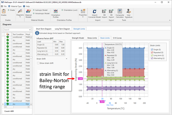
As explained above, the Bailey-Norton model can only represent the first and second creep phases (Figure 1). Therefore, the data range that is then used in the subsequent step to identify the model parameters usually has to be limited. The re-increase of the creep rate in the transition region from the second to the third creep phase is caused by an increasing damage of the material. In principle, the damage can be taken into account by including a damage term in the Bailey-Norton model [3]. However, this would then no longer be compliant with the original Bailey-Norton model and thus not easily applicable in a FEM program. In-house investigations with such an extended model show that the damage already starts early. It has been shown that the Bailey-Norton model still allows an acceptable fit of the model to the measured data up to a damage of approx. D = 1% (here the damage variable D is meant, not the strain!). Depending on the applied creep stress, this limiting damage then occurs at different times (Figure 4, green dots). What can also be seen, however, is that the range of the associated "limit strains" is comparatively narrow (Figure 4, green dots, left). Now, since in practice the value of the damage variable D is not known, as an approximation a long-term specific limiting strain for a commercial grade can be determined by means of MatScape as a substitute (Figure 5).
Step 3: Determination of the model parameters (calibration)
The material model is calibrated on the basis of Eq. (2), i.e. the creep curves and not the creep rate curve Eq. (1). The creep curves from step 1 considering step 2 can be used directly. Whereas fitting the model parameters to the creep rate curve can be numerically difficult if the creep curves are provided in the form of discrete data points. Differentiation of the creep strain with respect to time often causes scattering of the data points. As a rule, acceptable fitting results can then only be obtained by prior smoothing or analytical description of the creep curves.
The integration constant in Eq. (2) is theoretically zero, since at time t=0 the creep stress is also zero. By logarithmization, Eq. (2) can then be represented in linear form:
![]() (3)
(3)
Thus, a fit via a simple multiple linear regression is possible. However, this requires that the instantaneous strains that occur when the respective creep stress is applied are subtracted from the measured creep curves, so that the mere creep strains remain. Creep curves at at least two different creep stresses must be available to account for the dependence on stress. The model parameters must be determined by simultaneous fitting, taking all creep curves into account. Mathematically, the model parameters describe a 3D surface with the x-y axes time and stress and the z-axis strain. The determined model parameters B, n, s then describe the creep behavior within the parameter space.
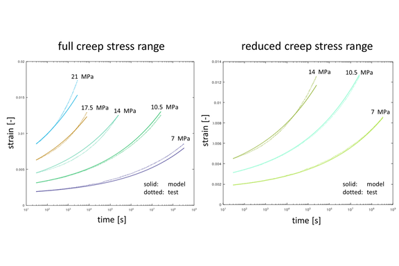
Figure 6 shows the result of a fitted model. In Figure 6, left, five creep curves in the range of 7 MPa to 21 MPa were used. In Figure 6, right, only three creep curves in the range of 7 MPa to 14 MPa were used for calibration. It can be clearly seen that the goodness of fit is worse with the larger creep stress range (Figure 6, left). This is caused by the fact that the creep curves at the higher creep stresses already reach the region of more severe damage. This can no longer be represented by the Bailey-Norton model, and the goodness of fit of the overall model is reduced compared to the restricted creep stress range (Figure 6, right). For practical applications, it can be deduced from this that the range of creep stresses used for calibration should not be too far away from the assumed stress range in the component. Calibration stresses chosen too high unnecessarily reduce the goodness of fit.
The assumption made above that the integration constant in Eq. (2) is zero is only true under ideal conditions. In the practical execution of the creep test, the creep stress can never be imposed within a theoretical zero time (step function). In this respect, the time period until the creep stress is reached is not accurately represented experimentally. A mixed state of time-independent instantaneous elastic and plastic strains and time-dependent viscous strains is present here. The application of nonlinear fitting methods such as the Levenberg-Marquardt method or gradient-free simplex methods can then lead to better fitting results than simple linear regression methods.
Step 4: Model validation and execution of the FEM simulation
All creep models, including the Bailey-Norton model, describe ideal visco-plastic material behavior. Once time-dependent plastic strains (viscous strains) have occurred, they do not recover when the load is removed and remain in the material. This means that these models are only suitable for monotonically increasing loads (i.e. constant or increasing loads), such as components under load-controlled force or pressure. The model can also be used for relaxation processes, i.e. deformation-controlled analyses. However, this is not considered further here.
Basically, the simulation requires two steps. In a first time-independent step, the load is applied. In a subsequent second step, the load is kept constant and the time-dependent deformation of the component under this load is calculated. Attention should be paid to the application of the load in the first step of the simulation. The material model for this can be either elastic or elasto-plastic. If the load or the resulting stresses in the component are comparatively high, i.e. reach the range of plastic deformations, the model should be elasto-plastic. The elasto-plastic material model used must then be consistent with the creep model used. I.e. in the context of a model validation by recalculation the creep test, the first strain values at time t1 > 0 of the underlying measured creep curves, per creep stress must be reached at the end of the first step of the simulation. The creep process then starts from there. Since creep models are time-dependent material models, the time increment used in the FEM analysis must be interpreted physically. For example, if the material model is calibrated in the unit of seconds, the FEM analysis must also be carried out in this time unit. Likewise, the time bases for applying the load in the first step and the creep in the second step must be matched to each other.
Step 5: Assessment
In the course of the material model calibration described above, assumptions were made that influence the interpretation of the simulation results. The objective of an FEM analysis with a creep model, is the representation of a time-dependent deformation history of a component or the determination of the time of component failure under long-term load. If necessary, both aspects are also of interest.
First, it is considered to what extent the obtained deformations or strains are reliable. One of the main limitations made was that the Bailey-Norton model is only valid up to a certain estimated limit strain or time per creep stress. Beyond this point, damage phenomena become increasingly dominant. The calculated strains lag behind the actual strains. In terms of component deformation, the model is therefore, strictly speaking, only valid up to the shortest calibration time or creep curve used. In the component, the strain distribution should be taken into account; if only small areas of the component, e.g. in notches, are stressed beyond the assumed limit strain, these highly stressed areas tend to have less influence on the overall component deformation. If, on the other hand, entire load-bearing cross-sections are subjected to overcritical strains, a more rigorous interpretation of the validity limits of the model must be applied.
With respect to the onset of failure due to yielding or fracture, other considerations must be made. A creep load case is a load-controlled analysis, i.e. the load (force, pressure) is prescribed and the deformation results. Thus, it can be approximately assumed that the stress is correctly calculated at any time and at any location in the component. Stress redistributions due to deformations are not taken into account. However, strains or deformations beyond the calibration range of the material model are not calculated correctly, as already explained in the previous section. However, this allows an assessment of the onset of failure for locally (approximately) correctly calculated stresses. The relevant material curve required for this is the so-called creep rupture diagram (Figure 2, bottom left). If the creep test has been carried out up to the point of failure, the measured failure times can be determined for each creep stress and plotted against each other. If such a diagram is available and a local component stress is available from the FEM analysis, a corresponding failure time can be determined via the creep rupture diagram. In this way, a life contour plot can be generated. In practice, however, a frequent problem is that such a creep diagram does not exist, since its determination is naturally very time-consuming.
Conclusion
Although the procedure for calibrating a Bailey-Norton creep model is presented in a structured way in this article, as so often, the devil is in the details. The effort required to calibrate is considerable. If the process is not practiced or has not been implemented in software, the execution is inefficient and error-prone. Under these conditions, it is more advisable to perform estimating analyses within the framework of optimization or concept studies on the basis of simple FEM simulations with linear-elastic or elastic-plastic isotropic material models. Procedures for this are presented in our blog article "Simulation of the Long-Term Behavior of Plastic Components".
If the use of a creep model is nevertheless unavoidable, future versions of our MatScape material modeling module integrated into the Converse and S-Life Plastics software products will support the calibration process outlined above. Converse and S-Life Plastics can be acquired either directly through PART Engineering or also through the Altair Partner Alliance. We are also happy to support you in the experimental determination of creep curves with accelerated test methods. Feel free to contact us.
[1] CAMPUS - a material information system for the plastics industry.
[2] M. Stommel, M. Stojek, und W. Korte: FEM zur Berechnung von Kunststoff- und Elastomerbauteilen, 2. Aufl. München: Carl Hanser Verlag, 2018
[3] W. Korte, F. Achereiner: Computational and Experimental Determination of Long-Term Material Properties for Plastics, NAFEMS World Congress, Tampa, Florida, USA, 2023
Author: Dr. Wolfgang Korte is Managing Director at PART Engineering GmbH, Bergisch Gladbach, Germany


